So, after sharing my post from last week about probabilities and stat arrays. Now, the way I determine which array is better is clearly overly arbitrary. Under that system the standard array is better than an array of (7, 18, 18, 18, 18, 18), when in reality any player looking for maximal stats would take that over the standard array (8, 10, 12, 13, 14, 15). So maybe there is a different way to compare these.
Now the first approach would be to just take the ability modifier. Each integer from 3-18 maps to an integer from -4 to +4 that is used for almost everything in the game (except for carrying capacity, which uses the actual Strength score).
Now this is great, however I want to be thorough. While in terms of in-game actions, a 10 is no different from an 11, having a higher score makes it easier to bump up the Ability Modifier later when a character gets leveled. So let’s use a modified scale. For the purpose of this, lets use a scale I found for 3.5E Dungeons and Dragons that I found while writing last week.
So, we’ll skip the simulation this week, and let’s start by generating our data table along with the sum of ability modifiers for each array:
library(tidyverse)## ── Attaching packages ─────────────────────────────────────── tidyverse 1.3.1 ──## ✓ ggplot2 3.3.3 ✓ purrr 0.3.4
## ✓ tibble 3.1.2 ✓ dplyr 1.0.6
## ✓ tidyr 1.1.3 ✓ stringr 1.4.0
## ✓ readr 1.4.0 ✓ forcats 0.5.1## ── Conflicts ────────────────────────────────────────── tidyverse_conflicts() ──
## x dplyr::filter() masks stats::filter()
## x dplyr::lag() masks stats::lag()statCombinations <- vector(mode = "list", length = 54264)
statPermutations <- vector(mode = "logical", length = 54264)
statOdds <- vector(mode = "logical", length = 54264)
sumModifier <- vector(mode = "logical", length = 54264)
sumModifier_human <- vector(mode = "logical", length = 54264)
maxPermutations <- factorial(6)
statRoll <- expand.grid(rep(list(1:6), 4))
statRoll <- apply(statRoll,1,sort)
dicepdf <- summary(as.factor(colSums(statRoll[2:4,])))/(6^4)
rolledStats <- c(15, 17, 16, 15, 17, 15)
rolledStats <- sort(rolledStats)
modifierVal <- function(a) {
modifiers <- as.list(floor((c(3:19) - 10)/2))
names(modifiers) <- c(3:19)
modifier <- 0
for (i in a) {
modifier <- modifier + as.numeric(modifiers[as.character(i)])
}
return(modifier)
}
diceodds <- function(a) {
probability <- 1
for (i in a) {
probability <- probability * as.numeric(dicepdf[as.character(i)])
}
return(probability)
}
pct_sum <- function(..., na.rm = FALSE) {
sum(..., na.rm = na.rm) * 100
}
counter <- 0
for (i1 in 3:18) {
pos1 <- i1
for (i2 in i1:18) {
pos2 <- i2
for (i3 in i2:18) {
pos3 <- i3
for (i4 in i3:18) {
pos4 <- i4
for (i5 in i4:18) {
pos5 <- i5
for (i6 in i5:18) {
pos6 <- i6
counter <- counter + 1
statCombinations[[counter]] <- c(pos1, pos2, pos3, pos4, pos5, pos6)
sumModifier[counter] <- modifierVal(statCombinations[[counter]])
sumModifier_human[counter] <- modifierVal(statCombinations[[counter]] + 1)
statOdds[counter] <- diceodds(statCombinations[[counter]])
statPermutations[counter] <- maxPermutations / prod(factorial(summary(as.factor(statCombinations[[counter]]))))
}
}
}
}
}
}
finaldf <- as_tibble(cbind(matrix(unlist(statCombinations), ncol = 6, byrow = T), statOdds, statPermutations, sumModifier, sumModifier_human)) %>%
mutate(probability = statOdds * statPermutations)## Warning: The `x` argument of `as_tibble.matrix()` must have unique column names if `.name_repair` is omitted as of tibble 2.0.0.
## Using compatibility `.name_repair`.So, taking our hypothesized array of (15, 17, 16, 15, 17, 15), let’s compare the odds we got last week with this new method. First, the old method:
finaldf %>%
  filter(V1 >= rolledStats[1] & V2 >= rolledStats[2] & V3 >= rolledStats[3] & V4 >= rolledStats[4] & V5 >= rolledStats[5] & V6 >= rolledStats[6]) %>%
  summarize_at(vars(probability),
               list(total_percent = pct_sum))
## # A tibble: 1 x 1
## total_percent
## <dbl>
## 1 0.00665This is 0.0066%, like we had last week. Now lets do the new way when comparing the sum total of ability modifiers:
finaldf %>%
  filter(sumModifier >= modifierVal(rolledStats)) %>%
  summarize_at(vars(probability),
               list(total_percent = pct_sum))
## # A tibble: 1 x 1
## total_percent
## <dbl>
## 1 0.268This time we get 0.2684%. This is a lot higher than the previous way, over 40 times in fact. However, even with that, it’s still less than a 1% chance, so I still would say it’s likely to be a cheating player (though that conclusion is not so strong as the old method).
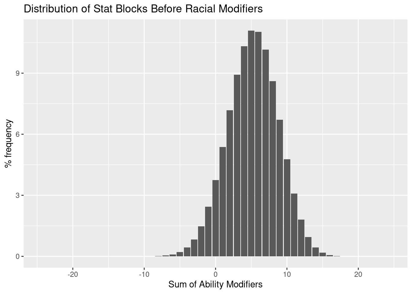
One thing this new method allows, is a lot mor intuition on what arrays are “better” than others, as well as to plot the distribution of these stat arrays. Lets plot this distribution.
modifierdist <- finaldf %>%
  group_by(sumModifier) %>%
  summarize_at(vars(probability), list(total_percent = pct_sum))

modifierdist %>%
  ggplot(aes(x = sumModifier, y = total_percent)) +
  geom_bar(stat = "identity") +
  ggtitle("Distribution of Stat Blocks Before Racial Modifiers") +
  ylab("% frequency") +
  xlab("Sum of Ability Modifiers")
The next thing we can do is we can actually calculate summary statistics using the definitions of median, mode, mean and standard deviation for discrete distributions like this. So let’s do it.
#median
modifierdist$sumModifier[50 <= cumsum(modifierdist$total_percent)][1]
## [1] 5#mode
modifierdist$sumModifier[which.max(modifierdist$total_percent)]## [1] 5#mean
sum(modifierdist$sumModifier * modifierdist$total_percent/100)## [1] 5.240741#standard deviation
sqrt(sum((modifierdist$sumModifier)^2 * modifierdist$total_percent/100) - (sum(modifierdist$sumModifier * modifierdist$total_percent/100))^2)## [1] 3.544196This gives a median and mode of +5, a mean of +5.2407, and a standard deviation of 3.5442.
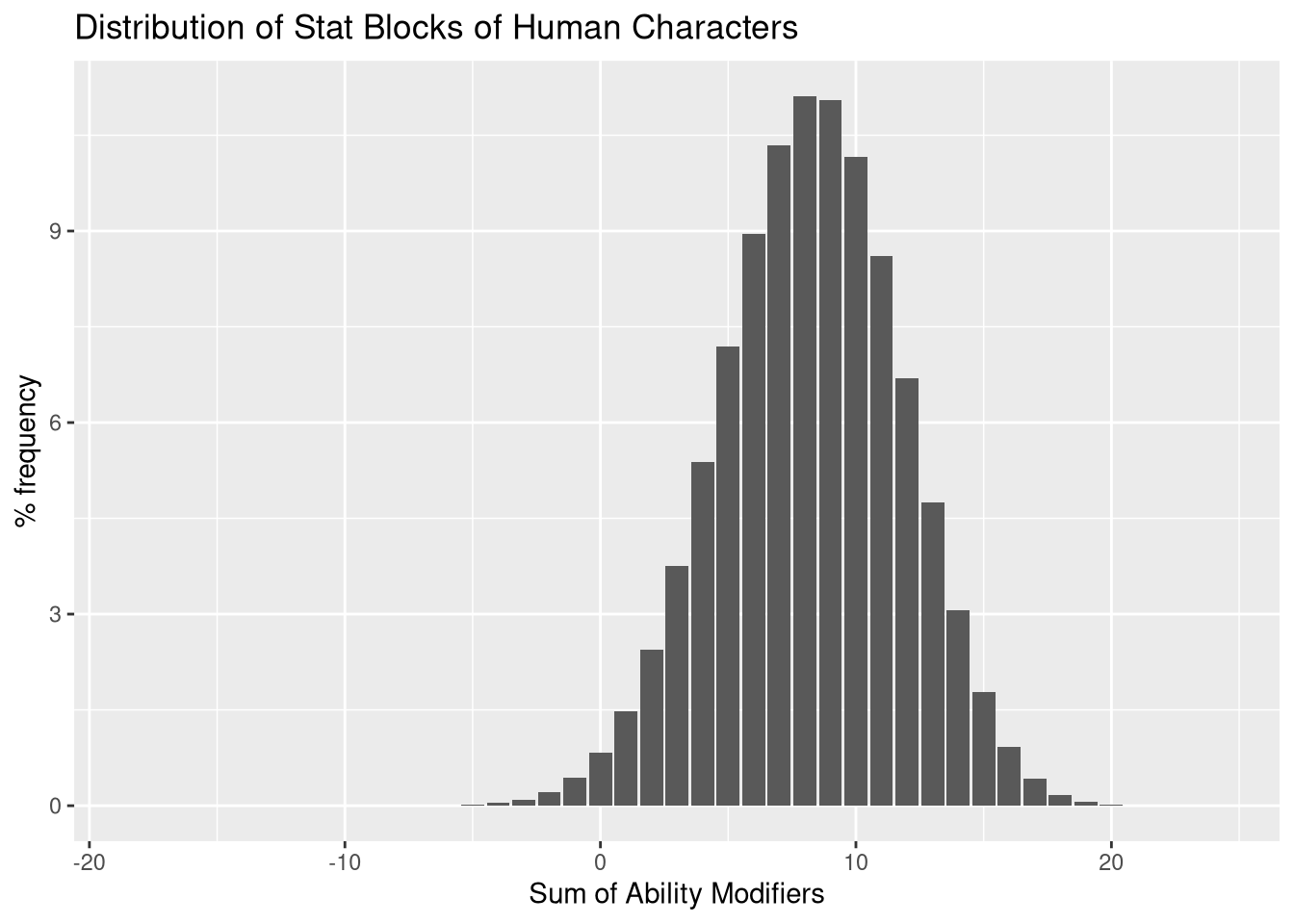
Now, these stats are only at the beginning of character creation. Based on the options chosen, at least two of your ability scores will increase, but doing this for all combinations is not so much practical. However, the most vanilla option is the Human option, which gives a +1 to each of your Ability Scores. So let’s take a look at that, plot the distribution and recalculate the summary statistics.
finaldf_human <- finaldf %>%
  mutate(V1 = V1 + 1, V2 = V2 + 1, V3 = V3 + 1, V4 = V4 + 1, V5 = V5 + 1, V6 = V6 + 1)

modifierdist_human <- finaldf_human %>%
  group_by(sumModifier_human) %>%
  summarize_at(vars(probability), list(total_percent = pct_sum))

modifierdist_human %>%
  ggplot(aes(x = sumModifier_human, y = total_percent)) +
  geom_bar(stat = "identity") +
  ggtitle("Distribution of Stat Blocks of Human Characters") +
  ylab("% frequency") +
  xlab("Sum of Ability Modifiers")
#median
modifierdist_human$sumModifier_human[50 <= cumsum(modifierdist_human$total_percent)][1]
## [1] 8#mode
modifierdist_human$sumModifier_human[which.max(modifierdist_human$total_percent)]## [1] 8#mean
sum(modifierdist_human$sumModifier_human * modifierdist_human$total_percent/100)## [1] 8.226852#standard deviation
sqrt(sum((modifierdist_human$sumModifier_human)^2 * modifierdist_human$total_percent/100) - (sum(modifierdist_human$sumModifier_human * modifierdist_human$total_percent/100))^2)## [1] 3.535849The median and mode are increased by 3 to +8. The mean also goes up around 3 to +8.2269, with the standard deviation being about the same at 3.5358
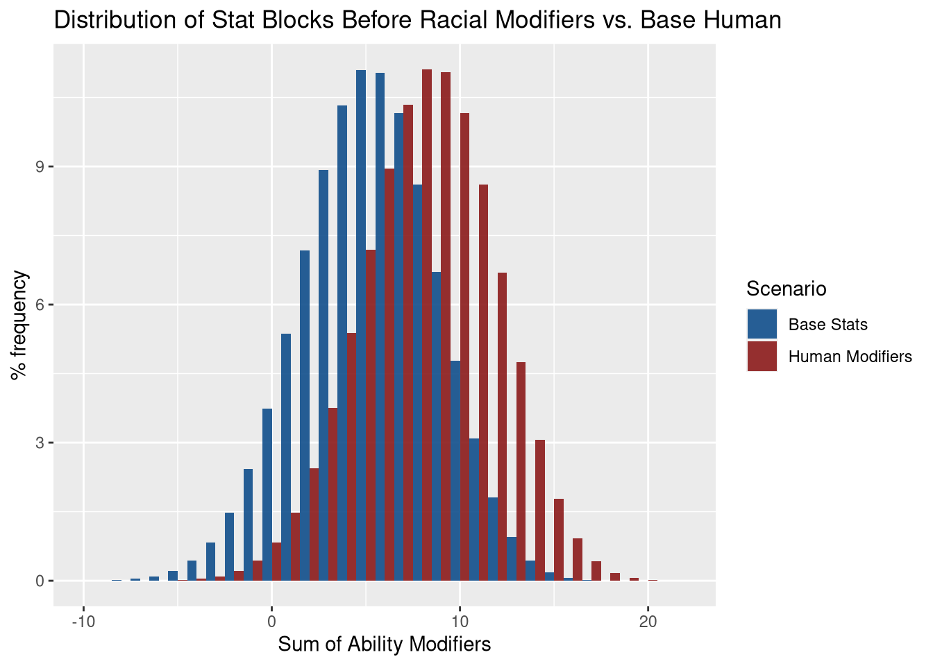
For completeness, let’s make one final graph with the base stats and the human option next to each other.
tmp1 <- finaldf %>%
  group_by(sumModifier_human) %>%
  summarize_at(vars(probability), list(total_percent = pct_sum))

tmp2 <- finaldf %>%
  group_by(sumModifier) %>%
  summarize_at(vars(probability), list(total_percent = pct_sum))

tmp3 <- rbind(tibble(sumModifier_human = rep(0,6), total_percent = rep(0,6)), tmp1)

comparedf <- tibble(sumModifier = tmp2$sumModifier, basePercent = tmp2$total_percent, humanPercent = tmp3$total_percent) %>%
  gather(`basePercent`, `humanPercent`, key = "type", value = "percent")

comparedf %>%
  ggplot() +
  geom_bar(aes(x = sumModifier, y = percent, fill = type), alpha = 0.9, width = 1, stat = "identity", position = position_dodge(width = 1)) +
  ggtitle("Distribution of Stat Blocks Before Racial Modifiers vs. Base Human") +
  ylab("% frequency") +
  xlab("Sum of Ability Modifiers") +
  xlim(-10, 22) +
  scale_fill_manual(name = "Scenario",labels = c("Base Stats", "Human Modifiers"), values = c("dodgerblue4", "firebrick4"))
## Warning: Removed 34 rows containing missing values (geom_bar).
We see that there’s about a +3 shift to the right, though if you look carefully it isn’t a simple shift of 3. For a simple example, the minimum value of the sum for base stats is -24, where for the Human option shifts that all the way to -18.